Step-By-Step Example to implement Parent-Child Hierarchy :
There are different types of hierarchy which exists in an Organization data which gives more insight for our analysis.
Ragged Hierarchy :A
hierarchy in which all the lowest-level members do not have the same
depth. For example, a Time hierarchy might have data for the current
month at the day level, the previous month’s data at the month level,
and the previous 5 years’ data at the quarter level. This type of
hierarchy is also known as an unbalanced hierarchy.
Skip-level Hierarchy :A
hierarchy in which certain members do not have values for certain
higher levels. For example, in the United States, the city of Washington
in the District of Columbia does not belong to a state. The expectation
is that users can still navigate from the country level (United States)
to Washington and below without the need for a state.
Parent-Child Hierarchy :Consists
of values that define the hierarchy in a parent-child relationship and
does not contain named levels. For example, an Employee hierarchy might
have no levels, but instead have names of employees who are managed by
other employees.
A parent-child hierarchy is a hierarchy of
members that all have the same type. This contrasts with level-based
hierarchies, where members of the same type occur only at a single level
of the hierarchy. The most common real-life occurrence of a
parent-child hierarchy is an organizational reporting hierarchy chart,
where the following all apply:
• Each individual in the organization is an employee.
• Each employee, apart from the top-level managers, reports to a single manager.
• The reporting hierarchy has many levels.
In
relational tables, the relationships between different members in a
parent-child hierarchy are implicitly defined by the identifier key
values in the associated base table. However, for each Oracle BI Server
parent-child hierarchy defined on a relational table, you must also
explicitly define the inter-member relationships in a separate
parent-child relationship table.
Let us start with Parent-Child Hierarchy and see how to implement it .
Am taking Employee table to work around . Click
here to download .sql file for Employee table DDL and Data .
Step1 : Create a blank repository and import the Employee table in to Physical Layer .

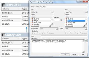
Step2: Create Alias on EMPLOYEE table 1.’EmployeeDim’ and
2.’SalaryFact’ and give physical join between EmployeeDim to SalaryFact .

Step3: Drag the tables in to BMM layer and give aggregations for the fact columns.

Step4: Now right click on Employees logical table and choose for new parent child hierarchy .
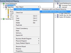
Step5:
Choose the member key (by default it will take the primary key . Here
Employee Number) and parent column as shown in the below screenshot.

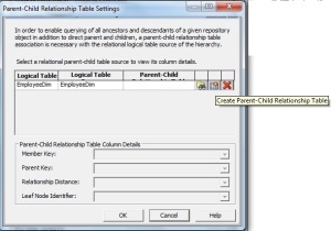
Step6:
Click on ‘parent- child settings’ .This is the place where we are going
to generate the DDL & DML scripts which we can use to create and
populate the hierarchy table which will be used by BI server to report
parent child hierarchies. Here click on ‘Create Parent-Child
Relationship Table’ .
Step7: Enter the DDL&DML script names and click Next .
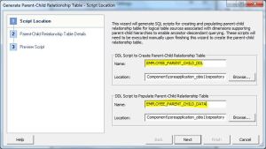
Step7: Give name for the Parent Child hierarchy table and Click Next .

Step8: You can see both DDL and Script to populate data here .

Click Finish .
You can see the screen as follows .

Click Ok again Ok .
After finishing the wizard you can see the HierarchyTable got imported automatically.
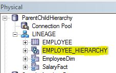
Right click on the EMPLOYEE_HIERARCHY table –> click on update
rowcount and observe that you will get ‘Table does not exist error’
Step9:Go
to the path
<beahome>\instances\instance1\bifoundation\OracleBIServerComponent\coreapplication_obis1\repository.
Run the scripts ‘EMPLOYEE_PARENT_CHILD_DDL.sql’ and
‘EMPLOYEE_PARENT_CHILD_DATA.sql’ .(My case I used SQL Developer to Run
this scripts)
DDL :
CREATE TABLE EMPLOYEE_HIERARCHY (
MEMBER_KEY DOUBLE PRECISION, ANCESTOR_KEY DOUBLE PRECISION, DISTANCE
NUMBER(10,0), IS_LEAF NUMBER(10,0) );
Script For polulate Data :
declare
v_max_depth integer;
v_stmt varchar2(32000);
i integer;
begin
select max(level) into v_max_depth
from EMPLOYEE
connect by prior EMP_NO=MANAGER_ID
start with MANAGER_ID is null;
v_stmt := ‘insert into LINEAGE.EMPLOYEE_HIERARCHY (MEMBER_KEY, ANCESTOR_KEY, DISTANCE, IS_LEAF)’ || chr(10)
|| ‘select EMP_NO as member_key, null, null, 0 from EMPLOYEE where MANAGER_ID is null’ || chr(10)
|| ‘union all’ || chr(10)
|| ‘select’ || chr(10)
|| ‘ member_key,’ || chr(10)
|| ‘ replace(replace(ancestor_key, ”\p”, ”|”), ”\”, ”\”) as ancestor_key,’ || chr(10)
|| ‘ case when depth is null then 0′ || chr(10)
|| ‘ else max(depth) over (partition by member_key) – depth + 1′ || chr(10)
|| ‘ end as distance,’ || chr(10)
|| ‘ is_leaf’ || chr(10)
|| ‘from’ || chr(10)
|| ‘(‘ || chr(10)
|| ‘ select’ || chr(10)
|| ‘ member_key,’ || chr(10)
|| ‘ depth,’ || chr(10)
|| ‘ case’ || chr(10)
|| ‘ when depth is null then ”” || member_key’ || chr(10)
|| ‘ when instr(hier_path, ”|”, 1, depth + 1) = 0 then null’ || chr(10)
||
‘ else substr(hier_path, instr(hier_path, ”|”, 1, depth) + 1,
instr(hier_path, ”|”, 1, depth + 1) – instr(hier_path, ”|”, 1, depth) –
1)’ || chr(10)
|| ‘ end ancestor_key,’ || chr(10)
|| ‘ is_leaf’ || chr(10)
|| ‘ from’ || chr(10)
|| ‘ (‘ || chr(10)
||
‘ select EMP_NO as member_key, MANAGER_ID as ancestor_key,
sys_connect_by_path(replace(replace(EMP_NO, ”\”, ”\”), ”|”, ”\p”), ”|”)
as hier_path,’ || chr(10)
|| ‘ case when EMP_NO in (select MANAGER_ID from EMPLOYEE ) then 0 else 1 end as IS_LEAF’ || chr(10)
|| ‘ from EMPLOYEE ‘ || chr(10)
|| ‘ connect by prior EMP_NO = MANAGER_ID ‘ || chr(10)
|| ‘ start with MANAGER_ID is null’ || chr(10)
|| ‘ ),’ || chr(10)
|| ‘ (‘ || chr(10)
|| ‘ select null as depth from dual’ || chr(10);
for i in 1..v_max_depth – 1 loop
v_stmt := v_stmt || ‘ union all select ‘ || i || ‘ from dual’ || chr(10);
end loop;
v_stmt := v_stmt || ‘ )’ || chr(10)
|| ‘)’ || chr(10)
|| ‘where ancestor_key is not null’ || chr(10);
execute immediate v_stmt;
end;
/
Click on COMMIT to commit changes .

Right click on the EMPLOYEE_HIERARCHY table –> click on update
rowcount and observe that you will not get ‘Table does not exist error’
.
Step10: Pull the ‘ParentChildHierarchy’ into Presentation
Layer ,Check Consistency and save the repository .Now we are ready to
Build reports .

Click
Here to download Repository (Repository Password : Admin123)
Step11: Go to answers create analysis including Employee Hierarchy . Thats it…
Reference:http://prasadmadhasi.com/2011/11/15/hierarchies-parent-child-hierarchy-in-obiee-11g/